Data vocabulary + univariate stats
Bivariate stats
Probability
Random variables
Bivariate distributions
100
The national time use survey was a random sample of US households asking how much time each member of the household spent on a variety of activities (working, cooking, cleaning, etc.) in a particular week.
True or False: This is an example of time-series data.
False
100
It is possible for two variables, x and y, to be related even in
s_{xy}
=0. True or False?
True
100
True or false: If events A and B are mutually exclusive, then P(B|A)=0.
True. If A happens, B cannot happen.
100
Let the discrete random variable X be given by the pdf below. This number is Var(X+3).
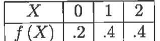
0.56
Var(X+3) = Var(X)
E(X) = 0*.2 + 1*.4 + 2*.4 = 1.2
E(X2)= 0*.2 + 1*.4 + 4*.4 =2
Var(X) = 2 - 1.22 =.56
100
True or False: If two random variables X and Y are independent, then the population slope, β1, is zero.
True. If two random variables are independent, there is no relationship between them, linear or otherwise.
200
This common transformation can make the distribution of a right-skewed variable more symmetric.
what is natural log transformation?
200
The following is STATA output from a least squares regression of standardized reading test scores at the end of kindergarten [stdreadk] on the number of days a student was absent in kindergarten [absentk]. This number is the SSM.
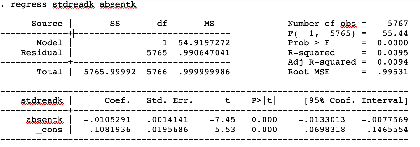
What is 55.06?
![]() .
.
200
You ask 5 randomly-chosen companies whether they have voluntarily implemented “green,” or environmentally-friendly, policies. Let X represent a variable that is set to 1 if a company is “green” and zero otherwise. Suppose that the probability that a company has gone “green” is p=0.4. This number is the probability of finding that exactly 4 companies in the sample have “green” policies.
What is 0.0768?
![]() .
.
200
Suppose that the variable x is drawn from a normal distribution with mean μ=0 and variance
\sigma^2=4
This is the value of c such that the probability that -c ≤ x ≤ c is approximately 0.997.
6.
This comes from the “rule of thumb” for calculating areas underneath the normal distribution. 99.7% of the data are within 3σ of μ. Thus, c=μ+3σ=6.
200
Consider two random variables X and Y, with Cov(X,Y)=3. This number is Cov(3X+2,5Y).
45
=Cov(3X+2,5Y)
=Cov(3X,5Y)
=15Cov(X,Y)
300
The exchange rate between the Great Britain pound (₤) and the Euro (€) was 1€ = 0.83₤. We gather a simple random sample of residents in each country and find that the sample average wealth in Great Britain (in ₤) is 0.75*sample average wealth in France (in €). The coefficient of variation of wealth in Great Britain is the same as the coefficient of variation of wealth in France.
True or false: The sample variance of wealth in France (in €) exceeds the sample variance of wealth in Great Britain (in ₤).
True. If the coefficient of variation (CV) of wealth in France is equal to the coefficient of variation of wealth in Great Britain, it must be the case the standard deviation of wealth in Great Britain = 0.75 * standard deviation of wealth in France. This implies that the variance of wealth in Great Britain=(0.75)2*variance of wealth in France. Said differently, the variance of wealth in Great Britain<variance of wealth in France.
300
Is the US a mobile society? To find out, Bhashkar Mazumder matched tax records of the earnings of parents and their children many years later. He regressed children’s ln(income) on parents’ ln(income) and estimated the a least squares slope of 0.61. Interpret the least squares slope.
The least squares slope implies that a 1% (10%) increase in parental income is on average associated with a 0.61% (6.1%) increase a child’s income. It is the elasticity of children’s income with respect to parents’ income.
300
P(A cap B) = 0.5, P(B) =.7, P(B|A)=0.7
Are A and B independent?
Yes
P(B) =P(B|A)
300
f(1.25) assuming
X~U[1,1.5]
2
300
True or false: Suppose that two random variables X and Y are such that E(XY)=0. This implies that there is no linear population relationship between X and Y.
False
400
Consider this table by Allen and Barnsley (1993), describing the birthdates of Canadian hockey players. “NHL” stands for the “National Hockey League” – the highest level of play in the world. “WHL” and “OHL” represent Canadian minor league hockey (the Western Hockey League, and the Ontario Hockey League, respectively). Supposing that birth quarter can be interpreted as a numerical variable (taking on the values of 1, 2, 3, and 4), calculate the sample mean birth quarter of NHL players in 1982-83 on the basis of the information presented in the table.
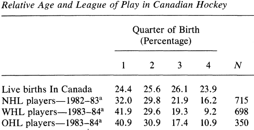
What is 2.22?
![]()
![]()
OR:
![]()
![]()
400
Consider three variables x, y, z. Assume
|r_{xy}|>|r_{zy}|
This implies that the error sum of squares (SSE) is lower for a regression of y on x than for a regression of y on z. True or False.
True.
400
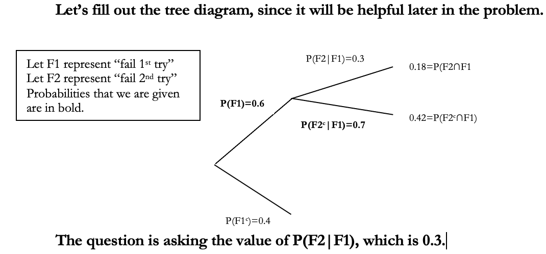
In some state, 40% of law school graduates pass the bar exam on their first try. Of those who fail the first time, 70% pass the second time they take the test. This number is the probability of failing the bar a second time, conditional on failing on the first attempt.
What is 0.3?
400
X is a random variable, with
X~N(0,1)
. This number is
P(X\geq2).
What is 0.025?
From the “68-95-99.7” rule, we know that 95% of values are within two standard deviations of the mean. Given symmetric, this implies that the probability that X is greater than 2 is approximately 0.025. (Or if you look at the normal distribution table, you would find the precise answer is 0.023.)
400
Suppose that X and Y are both Bernoulli random variables and that P(Y=0|X=1) = 0.4. This number is the expected value of Y given that X=1.
What is 0.6?
![]() . We know that
. We know that ![]() . Therefore,
. Therefore,![]()
500
Match the summary statistics to the histogram, for each of the 3 variables below.
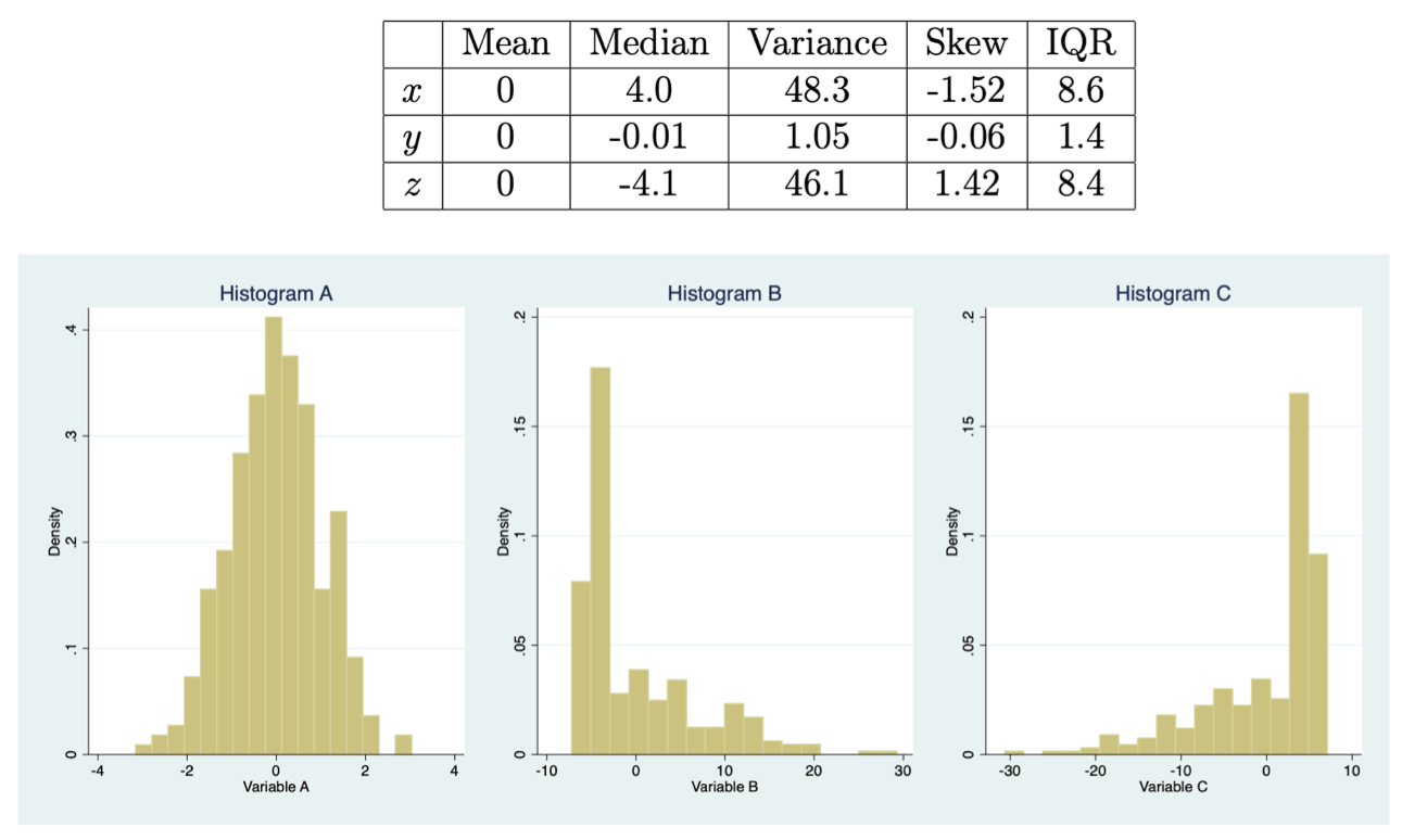
Histogram A = y
Histogram B = z
Histogram C = x
500
In Project STAR (“Student-Teacher Achievement Ratio”), students were randomly assigned to classes of different sizes at the start of kindergarten. The students were followed over time to estimate the causal impact of smaller classes on test performance and other academic outcomes. The Project STAR data do, however, contain information on other student characteristics. Researchers ran a least squares regression of standardized reading test scores at the end of kindergarten [stdreadk] on the number of days a student was absent in kindergarten [absentk].
Is the following statement true or false? Explain your answer: “Because Project STAR was an experiment, the least squares regression above tells us about the causal relationship between school absences and test performance.”
FALSE. Project STAR was an experiment, but it was not an experiment designed to estimate the causal effect of school absences. Said differently, school absences among Project STAR participants were not randomly assigned. As a result, children with more school absences might have other characteristics (e.g., parents who don’t value education, illness) that might also be related to test performance. The least squares slope in the above regression is “picking up” these influences, as well as the direct effect of missing school.
500
In some state, 40% of law school graduates pass the bar exam on their first try. Of those who fail the first time, 70% pass the second time they take the test. This number is the probability of passing the bar exam on either the first or second try.
what is 0.82?
![]()
500
You ask 5 randomly-chosen companies whether they have voluntarily implemented “green,” or environmentally-friendly, policies. Let X represent a variable that is set to 1 if a company is “green” and zero otherwise. Suppose that the probability that a company has gone “green” is p=0.4. This number is the standard deviation of
\overline{x}?
What is 0.22?
Let’s just calculate the right answer:
![]()
…using expectations rules. Since we have a random sample, the Xi’s are independent. Thus, the variance of this sum will contain no covariance terms (it will just be the sum of the variances):
![]() .
.
Thus, the standard deviation is ![]() .
.
500
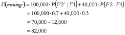
In some state, 40% of law school graduates pass the bar exam on their first try. Of those who fail the first time, 70% pass the second time they take the test.
Now suppose that law firms carried about whether a student passed the bar on the first try: students who pass the first time earn $150,000 a year in their first job, students who pass on their second attempt earn $100,000 a year, and those who fail both times work as paralegals for $40,000 a year.
This number is the expected earnings of a law student who failed the bar the first time
What is 82,000?
There are only two relevant outcomes are ![]() and
and ![]() , which occur with probabilities 0.7 and 0.3, respectively. Again, we use these probabilities as weights in calculating expected earnings:
, which occur with probabilities 0.7 and 0.3, respectively. Again, we use these probabilities as weights in calculating expected earnings: