An airline records data on several variables for each of its flights: model of plane, amount of fuel used, time in flight, number of passengers, and whether the flight arrived on time. The number and type of variables recorded are...?
Categorical = 2
Discrete Quant. = 1
Continuous Quant. = 2
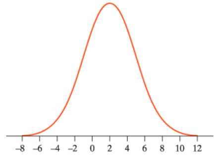
For the Normal distribution shown, the standard deviation is closest to...
a. 3
b. 0
c. 1
d. 2
e. 5
a. 3
Here are three residual plots of the same data transformed in different ways. Which of the three would be the most appropriate to make a line of least squared regression?
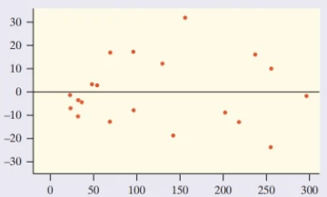
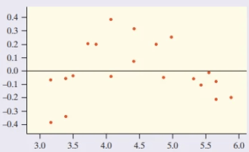
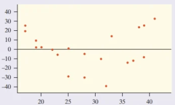
The residual plot for Option 1 is much more scattered, while the residual plots for Option 2 and 3 are obviously curved or roughly curved, meaning that the first model is the most appropriate.
Realtors collect data in order to serve their clients more effectively. In a recent week, data on the age of all homes sold in a particular area were collected. The standard deviation of the distribution of house age is about 16 years. Interpret this value.
The age of the houses in the sample typically varies by about 16 years from the mean age.
The Environmental Protection Agency (EPA) requires that the exhaust of each model of motor vehicle be tested for the level of several pollutants. The level of oxides of nitrogen (NOX) in the exhaust of one light truck model was found to vary among individual trucks according to an approximately Normal distribution with mean μ=1.45 grams per mile driven and standard deviation σ=0.40 gram per mile. Which of the following best estimates the proportion of light trucks of this model with NOX levels greater than 2 grams per mile?
Normalcdf(lower: 2, upper: 1000, mean: 1.45, SD: 0.4) = 0.0846 = 8.46%
The scatterplot shows the relationship between the number of people per television set and the number of people per physician for 40 countries, along with the least-squares regression line. In Ethiopia, there were 503 people per TV and 36,660 people per doctor. Which of the following is correct?
(a) Increasing the number of TVs in a country will attract more doctors.
(b) The slope of the least-squares regression line is less than 1.
(c) The correlation is greater than 1.
(d) The point for Ethiopia is decreasing the slope of the least-squares regression line.
(e) Ethiopia has more people per doctor than expected, based on how many people it has per TV.
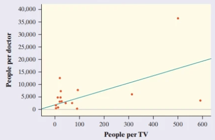
e. Ethiopia has more people per doctor than expected, based on how many people it has per TV.
Below is a table that summarizes data on survival status by gender and class of travel on the Titanic. Find the distributions of survival status for males and for females within each class of travel. Did women survive the disaster at higher rates than men? Explain.

First class
Female survived: 140/144 = 97.2%
Female died: 4/144 = 2.8%
Male survived:
57/175 = 32.6%
Male died: 118/175 = 67.4%
Second class
Female survived: 80/93 = 86%
Female died: 13/93 = 14%
Male survived: 14/168 = 8.3%
Male died: 154/168 = 91.7%
Third class
Female survived: 76/165 = 46.1%
Female died: 89/165 = 53.9%
Male survived: 75/462 = 16.2%
Male died: 387/462 = 83.8%
Regardless of class of travel, women survived the disaster at higher rates than men. Of those who were traveling first class, women were about 3 times more likely to survive than men. Of those who were traveling second class, women were about 10 times more likely to survive than men. Of those who were traveling third class, women were about 3 times more likely to survive than men.
Until the scale was changed in 1995, SAT scores were based on a scale set many years ago. For Math scores, the mean under the old scale in the early 1990s was 470 and the standard deviation was 110. In 2016, the mean was 510 and the standard deviation was 103. Gina took the SAT in 1994 and scored 500. Her cousin Colleen took the SAT in 2016 and scored 530. Who did better on the exam, and how can you tell?
Gina — her standardized score is higher than Colleen’s 0.27 > 0.13
Long-term records from the Serengeti National Park in Tanzania show interesting ecological relationships. When wildebeest are more abundant, they graze the grass more heavily, so there are fewer fires and more trees grow. Lions feed more successfully when there are more trees, so the lion population increases. Researchers collected data on one part of this cycle, wildebeest abundance (in thousands of animals), and the percent of the grass area burned in the same year.
(a) Give the equation of the least-squares regression line. Be sure to define any variables you use.
(b) What is the predicted value of percent of grass burned when there are 750k Wildebeasts
(c) Interpret the standard deviation of the residuals and r^2.
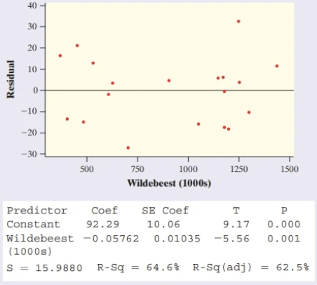
a. y = 92.29 - 0.05762x
b. y = 92.29 - 0.05762(750) = 49.075
c. The actual percentage of burned area is typically about 15.988% away from the percent predicted by the least-squares regression line with x = number of wildebeest (1000s). The value of r^2 = 64.6%. Interpretation: About 64.6% of the variability in percentage of burned area is accounted for by the least-squares regression line with x = number of wildebeest (1000s).
Forty students took a statistics test worth 50 points. The dotplot displays the data. Describe the distribution below.

I ran out of time to make this answer ¯\_(ツ)_/¯
For a certain online store, the distribution of the number of purchases per hour is approximately normal with a mean 1,200 purchases and a standard deviation of 200 purchases. What is the number of sales will be acquired in the top 22 percent of sales?
About 1,354 sales
Which of the following statements is not true of the correlation r between the lengths (in inches) and weights (in pounds) of a sample of brook trout?
(a) r must take a value between −1 and 1.
(b) r is measured in inches.
(c) If longer trout tend to also be heavier, then r > 0.
(d) r would not change if we measured the lengths of the trout in centimeters instead of inches.
(e) r would not change if we measured the weights of the trout in kilograms instead of pounds.
(b) r is measured in inches. Is FALSE because r is unit free
The American Statistical Association (ASA) has an Instagram account (@amstatnews). Bedford, Freeman & Worth (BFW), the publisher of this textbook, also has an Instagram account (@bfwhighschool). Below are the number of Instagram likes for 10 randomly selected posts from each account and numerical summaries of the data. Compare these distributions.
Shape: Both distributions of number of Instagram likes are slightly skewed to the right.
Outliers: There is one high outlier in the ASA distribution: the post with 16 likes. There is also one high outlier in the BFW distribution: the post with 38 likes.
Center: The BFW Instagram account had a higher median number of likes (17) than the ASA Instagram account (7.5). More importantly, 100% of the BFW posts had a number of likes greater than the median for the ASA account.
Variability: There is more variation in number of likes among the BFW posts than the ASA posts. The IQR for the BFW posts (5) is larger than the IQR for the ASA posts (4). TRM Do You Know Your Geography? Consider doing the activity, “Do you know your geography?,” found in the Teacher’s Resource Materials. The activity has each student answer a couple of questions about geography. However, there are two versions of the “geography quiz.”
The average yearly snowfall in Chillyville is approximately Normally distributed with a mean of 55 inches. If the snowfall in Chillyville exceeds 60 inches in 15% of the years, what is the standard deviation?
The value 1.04 is the approximate 85th percentile of the standard Normal distribution
Sarah’s parents are concerned that she seems short for her age. Their doctor has kept the following record of Sarah’s height.
a. Using your calculator, find the equation of the least-squares regression line.
b. Calculate and interpret the residual for the point when Sarah was 48 months old.
c. Would you be confident using the equation from part (a) to predict Sarah’s height when she is 40 years old? Explain.
a. The regression line for predicting y = height from x = age is y = 71.95 + 0.3833x.
b. At age 48 months, we predict Sarah’s height to be y = 71.95 + 0.3833(48) = 90.348 cm. The residual for Sarah is 90 - 90.348 = 0.348. Interpretation: Sarah’s actual height was 0.348 cm less than the height predicted by the regression line with x = 48 months.
c. No; obviously, the linear trend will not continue until she is 40 years old. Our data were based only on the first 5 years of life and predictions should only be made for ages 0–5.